DRAFT
Project Overview
- Goal: Help CharityML maximize the likelihood of receiving dontations
How: Construct a model that predicts whether an individual makes more than 50k/yr, a value associated with being a candidate for giving donations
Data Source: 1994 US Census Data UCI Machine Learning Repository
Note: Datset donated by Ron Kohavi and Barry Becker, from the article "Scaling Up the Accuracy of Naive-Bayes Classifiers: A Decision-Tree Hybrid". Small changes to the dataset have been made, such as removing the 'fnlwgt' feature and records with missing or ill-formatted entries.
Table of Contents:
1.1 Data Dictionary
1.2 Simple Cleaning
1.3 Summary Statistics
1.4 Distributions
1.5 Skew and Variance
1.6 Relationships
2.1 Separate Labels from Factors
2.2 Transformation2.2.1 Indicator Variables
2.2.2 Impact
2.2.3 Logarithmic Transform
2.2.4 Normalization and Standardization2.4 Pipeline
3.Metrics
3.1 Accuracy
3.2 Precision
3.3 Recall
3.4 F$\beta$-Score
4.Models
4.1 Selection
4.2.1 Application
4.3 Model Application Pipeline
4.4.1 Application
4.4.2 Tuning4.5 Random Forest
4.5.1 Application
4.5.2 Tuning4.6 Ada Boost
4.6.1 Application
4.6.2 Tuning4.7 Gradient Boost
4.7.1 Application
4.7.2 Tuning4.8.1 Application
4.8.2 Tuning4.9.1 Application
4.9.2 Tuning4.10 Comparison
4.10.1 Feature Importance
4.10.2 Selection
4.10.3 Comp: Reduced Feature Model Performance
5.Summary
1.1 EDA: Data Dictionary
- age: continuous.
- workclass: Private, Self-emp-not-inc, Self-emp-inc, Federal-gov, Local-gov, State-gov, Without-pay, Never-worked.
- education_level: Bachelors, Some-college, 11th, HS-grad, Prof-school, Assoc-acdm, Assoc-voc, 9th, 7th-8th, 12th, Masters, 1st-4th, 10th, Doctorate, 5th-6th, Preschool.
- education-num: continuous.
- marital-status: Married-civ-spouse, Divorced, Never-married, Separated, Widowed, Married-spouse-absent, Married-AF-spouse.
- occupation: Tech-support, Craft-repair, Other-service, Sales, Exec-managerial, Prof-specialty, Handlers-cleaners, Machine-op-inspct, Adm-clerical, Farming-fishing, Transport-moving, Priv-house-serv, Protective-serv, Armed-Forces.
- relationship: Wife, Own-child, Husband, Not-in-family, Other-relative, Unmarried.
- race: Black, White, Asian-Pac-Islander, Amer-Indian-Eskimo, Other.
- sex: Female, Male.
- capital-gain: continuous.
- capital-loss: continuous.
- hours_per-week: continuous.
- native-country: United-States, Cambodia, England, Puerto-Rico, Canada, Germany, Outlying-US(Guam-USVI-etc), India, Japan, Greece, South, China, Cuba, Iran, Honduras, Philippines, Italy, Poland, Jamaica, Vietnam, Mexico, Portugal, Ireland, France, Dominican-Republic, Laos, Ecuador, Taiwan, Haiti, Columbia, Hungary, Guatemala, Nicaragua, Scotland, Thailand, Yugoslavia, El-Salvador, Trinadad&Tobago, Peru, Hong, Holand-Netherlands.
1.2 EDA: Simple Cleaning and Engineering
Standardizing factor names by PEP8 Naming Convention Standards can be helpful.
There are a number of categorical variables. Handling those with one-hot encoding can be helpful.

1.5 EDA: Skew and Variance
The features capital_gain and capital_loss are positively skewed (i.e. have a long tail in the positive direction).
To reduce this skew, a logarithmic transformation, $\tilde x = \ln\left(x\right)$, can be applied. This transformation will reduce the amount of variance and pull the mean closer to the center of the distribution.
Why does this matter: The extreme points may affect the performance of the predictive model.
Why care: We want an easily discernible relationship between the independent and dependent variables; the skew makes that more complicated.
Why DOESN'T this matter: The distribution of the independent variables is not an assumption of most models, but the distribution of the residuals and homoskedasticity of the independent variable, given the independent variables, $E\left(u | x\right) = 0$ where $u = Y - \hat{Y}$ is of linear regression. In this analysis, the dependent variable is categorical (i.e. discrete or non-continuous) and linear regression is not an appropriate model.
1.6 EDA: Relationships
Toward determing what factors should be included in the model, there is something to note with regard to categorical versus continuous variables.
Correlation is defined as: $$r = \frac{\sum\left(X-\bar{X}\right)\cdot\left(Y-\bar{Y}\right)}{\sqrt{(\sum\left(X-\bar{X}\right)^{2})}\cdot\sqrt{\sum\left(Y-\bar{Y}\right)^{2}}}$$
This is inconsistent with categorical variables. Instead, it can be useful to utilize the uncertainty coefficient, or Thiel's Index.
Where we have entropy of a single distribution:
$$H\left(X\right)=-\sum_{x} P_{x}\left(x\right)log\ P_{x}\left(x\right)$$Conditional entropy as:
$$H\left(X|Y\right) = - \sum_{x,y} P_{X,Y}\left(x,y\right)log\ P_{X|Y}\left(x|y\right)$$and the uncertainty coefficient as:
$$U\left(X|Y\right)=\frac{H\left(x\right)-H\left(X|Y\right)}{H\left(X\right)} = \frac{I\left(X;Y\right)}{H\left(X\right)}$$Where $I\left(X;Y\right)$ is the mutual information, or the amount of information obtained about one random variable through observing the other random variable.
To quote Shaked Zychlinski, "given the value of x, how many possible states does y have, and how often do they occur".
So, can this help us discenr some information about what to do with our factors?
I will step forward now with the idea that colinearity, where one variable can easily be derived from another within the model, is not desired (i.e. two variables with strong relationships on one another should not be included as they may reduce the predictive power of the model).
Citation: Shaked Zychlinski
Notable relationships
A model including:
ageandmarital_status(0.56)age&incomeis 0.24marital_status&incomeis 0.20
dropmarital_status
ageandrelationship(0.46)ageandincomeis 0.24relationshipandincomeis 0.21- drop
relationship
education_numandoccupation(0.57)education_numandincomeis 0.33occupationandincomeis 0.11- drop
occupation
marital_statusandrelationship(0.49)- already determined that
marital_statusandrelationshipwould be dropped from model
- already determined that

2. Data Engineering
2.1 Separate Labels from Factors
2.2 Transformation
2.2.1 Indicator Variables
2.2.2 Logarithmic Transform
2.2.3 Impact
2.2.4 Normalization and Standardization
2.1 DE: Separate Labels from Factors
For training an algorithm, it is useful to separate the label, or dependent variable ($Y$) from the rest of the data training_features, or independent variables ($X$).
2.2.1 DE: Indicator Variables
A common way to handle categorical variables is to make indicator, or dummy, variables from the values of the factors.
Pandas has a simple method, .get_dummies(), that can perform this very quickly.
Further, this will create a new variable for every value a categorical variable takes as demonstrated in this example:
| someFeature | someFeature_A | someFeature_B | someFeature_C | ||
|---|---|---|---|---|---|
| 0 | B | 0 | 1 | 0 | |
| 1 | C | ----> one-hot encode ----> | 0 | 0 | 1 |
| 2 | A | 1 | 0 | 0 |
Which means the p, or number of factors, will grow, and can do so potentially in a large way. Specifically, if p is the number of factors and pI is the number of factors after creating indicator variables:
$$pI = p + \left(number\ of\ distinct\ categories\right) \cdot \left(number\ of\ categorical\ variables\right)$$
It is also worth noting that for modeling, it is important that once value of the factor, a "base case", be dropped from the data. This is because the base case is redundant, i.e. can be infered perfectly from the other cases, and, more specifically and more detrimental to our model, it leads to multicollinearity of the terms.
In some models (e.g. logistic regression, linear regression), an assumption of no multicollinearity must hold.
So, the final number of factors after creating indicator variables and dropping the base case is: $$\tilde{p}=pI - \left(number\ of\ categorical\ variables\right)$$
2.2.2 DE: Logarithmic Transform
To reduce skew, a logarithmic transformation, $\tilde x = \ln\left(x\right)$, can be applied. This transformation will reduce the amount of variance and pull the mean closer to the center of the distribution.
The logarithmic transformation reduced the skew and the variance of each factor.
| Feature | Skewness | Mean | Variance |
|---|---|---|---|
| Capital Loss | 4.516154 | 88.595418 | 163985.81018 |
| Capital Gain | 11.788611 | 1101.430344 | 56345246.60482 |
| Log Capital Loss | 4.271053 | 0.355489 | 2.54688 |
| Log Capital Gain | 3.082284 | 0.740759 | 6.08362 |
2.2.3 DE: Impact
Originally, the influence of capital_loss on income was statistically significant, but after the logarithmic transformation, it is not.
Here it can be seen that with a change to the skew, the confidence interval now passes through zero whereas before it did not.
This passing through zero is interpreted as the independent variable being statistically indistinguishable from zero influence on the dependent variable.
2.2.4 DE: Normalization and Standardization
These two terms, normalization and standardization, are frequently used interchangably, but have two different scaling purposes.
- Normalization: scale values between 0 and 1
- Standardization: transform data to follow a normal distribution, i.e. $X \sim N\left(\mu=0,\sigma ^{2}=1\right)$
Earlier, capital_gain and capital_loss were transformed logarithmically, reducing their skew, and affecting the model's predictive power (i.e. ability to discern the relationship between the dependent and independent variables).
Another method of influencing the model's predictive power is normalization of independent variables which are numerical. Whereafter, each featured will be treated equally in the model.
However, after scaling is applied, observing the data in its raw form will no longer have the same meaning as before.
Note the output from scaling. age is no longer 39 but is instead 0.30137. This value is meaningful only in context of the rest of the data and not on its own.
2.3 DE: Shuffling and Splitting
After transforming with one-hot-encoding, all categorical variables have been converted into numerical features. Earlier, they were normalized (i.e. scaled between 0 and 1).
Next, for training a machine learning model, it is necessary to split the data into segments. One segment will be used for training the model, the training set, and the other set will be for testing the mode, the testing set.
A common method of splitting is to segment based on proportion of data. A general 80:20 rule is typical for training:test.
sklearn has a method that works well for this, .model_selection.train_test_split. Essentially, this randomly selects a portion of the data to segment to a training and to a testing set.
random_state: By setting a seed, optionrandom_state, we can ensure the random splitting is the same for our model. This is necessary for evaluating the effectiveness of the model. Otherwise, we would be training and testing a model with the same proportional split (if we kept that static), but with different observations of the data.test_size: This setting represents the proportion of the data to be tested. Generally, this is the complement (1 - x = c) of thetraining_size. For example, iftest_sizeis0.2, thetest_sizeis0.8.stratify: Preserves the proportion of the label class in the split data. As an example, let1and0indicate the positive and negative cases of a label, respectively. It's possible that only positive or only negative classes exisst in either training or testing set (e.g. $\forall y \in Y_{train}, y = 1$). Better than avoid this worst case scenario,stratifywill preserve the ratio of positive to negative classes in each training and testing set.
Here the data is split 80:20 with a seed set of 0 and the distribution of the label's classes preserved:
3. Metrics
3.1 Accuracy
3.2 Precision
3.3 Recall
3.4 F$\beta$-Score
In terms of income as a predictor for donating, CharityML has stated they will most likely receive a donation from individuals whose income is in excess of 50,000/yr.
CharityML has limited funds to reach out to potential donors. Misclassifying a person as making more than 50,000yr is COSTLY for CharityML. It's more important that the model accurately predicts a person making more than 50,000/yr (i.e. true-positive) than accidentally predicting they do when they don't (i.e. false-positive).
3.1 Met: Accuracy
Accuracy is a measure of the correctly predicted data points to total amount of data points:
$$Accuracy=\frac{\sum Correctly\ Classified\ Points}{\sum All\ Points}=\frac{\sum True\ Positives + \sum True\ Negatives}{\sum Observations}$$A Confusion Matrix demonstrates what a true/false positive/negative is:
| Predict 1 | Predict 0 | |
|---|---|---|
| True 1 | True Positive | False Negative |
| True 0 | False Positive | True Negative |
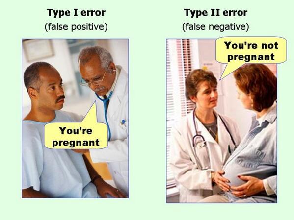
The errors of these are sometimes refered to as type errors:
| Predict 1 | Predict 0 | |
|---|---|---|
| True 1 | True Positive | Type 2 Error |
| True 0 | Type 1 Error | True Negative |
- Type 1: a positive class is predicted for a negative class (false positive)
- Type 2: a negative class is predicted for a positive class (false negative)
For this analysis, we want to avoid false positives or type 1 errors. Put differently, we prefer false negatives to false positives.
A model that meets that criteria, $False\ Negative \succ False\ Positive$, is known as preferring precision over recall, or is a high precision model.
Humorously and perhaps more understandably, these type errors can be demonstrate as such:
3.2 Met: Precision
Precision is a measure of the amount of correctly predicted positive class to the amount of positive class predictions (correct as well as incorrect predictions of positive class):
$$Precision = \frac{\sum True\ Positives}{\sum True\ Positives + \sum False\ Positives}$$A model which avoids false positives would have a high precision value, or score. It may also be skewed toward false negatives.
3.3 Met:Recall
Recall, sometimes refered to as a model's sensitivity, is a measure of the correctly predicted positive classes to the actual amount of positive classes (true positive and false negatives are each actual positive classes):
$$Recall = \frac{\sum True\ Positives}{\sum Actual\ Positives} = \frac{\sum True\ Positives}{\sum True\ Positives + \sum False\ Negatives}$$A mode which avoids false negatives would have a high recall value, or score. It may also be skewed toward false positives
3.4 Met: F-$\beta$ Score
An F-$\beta$ Score is a method of scoring a model both on precision and recall.
Where $\beta \in [0,\infty)$:
$$F_{\beta} = \left(1+\beta^{2}\right) \cdot \frac{Precision\ \cdot Recall}{\beta^{2} \cdot Precision + Recall}$$When $\beta = 0$, we get precision: $$F_{\beta=0} = \left(1+0^{2}\right) \cdot \frac{Precision\ \cdot Recall}{0^{2} \cdot Precision + Recall} = \left(1\right) \cdot \frac{Precision\ \cdot Recall}{Recall} = Precision$$
When $\beta = 1$, we get a harmonized mean of precision and recall:
$$F_{\beta=1} = \left(1+1^{2}\right) \cdot \frac{Precision\ \cdot Recall}{1^{2} \cdot Precision + Recall} = \left(2\right) \cdot \frac{Precision\ \cdot Recall}{Precision + Recall}$$- Note: $Harmonic\ Mean = \frac{2xy}{x + y}$
... and when $\beta > 1$, we get something closer to recall:
$$F_{\beta \rightarrow \infty} = \left(1+\beta^{2}\right) \cdot \frac{Precision\ \cdot Recall}{\beta^{2} \cdot Precision + Recall} = \frac{Precision\ \cdot Recall}{\frac{\beta^{2}}{1+\beta^{2}} \cdot Precision + \frac{1}{1+ \beta^{2}} \cdot Recall}$$As $\beta \rightarrow \infty$: $$\frac{Precision\ \cdot Recall}{\frac{\beta^{2}}{1+\beta^{2}} \cdot Precision + \frac{1}{1+ \beta^{2}} \cdot Recall} \rightarrow \frac{Precision \cdot Recall}{1 \cdot Precision + 0 \cdot Recall} = \frac{Precision}{Precision} \cdot Recall = Recall$$
4. Models
4.1 Selection
4.2.1 Application
4.3 Model Application Pipeline
4.4.1 Application
4.4.2 Tuning4.5 Random Forest
4.5.1 Application
4.5.2 Tuning4.6 Ada Boost
4.6.1 Application
4.6.2 Tuning4.7 Gradient Boost
4.7.1 Application
4.7.2 Tuning4.8.1 Application
4.8.2 Tuning4.9.1 Application
4.9.2 Tuning4.10 Comparison
4.10.1 Feature Importance
4.10.2 Selection
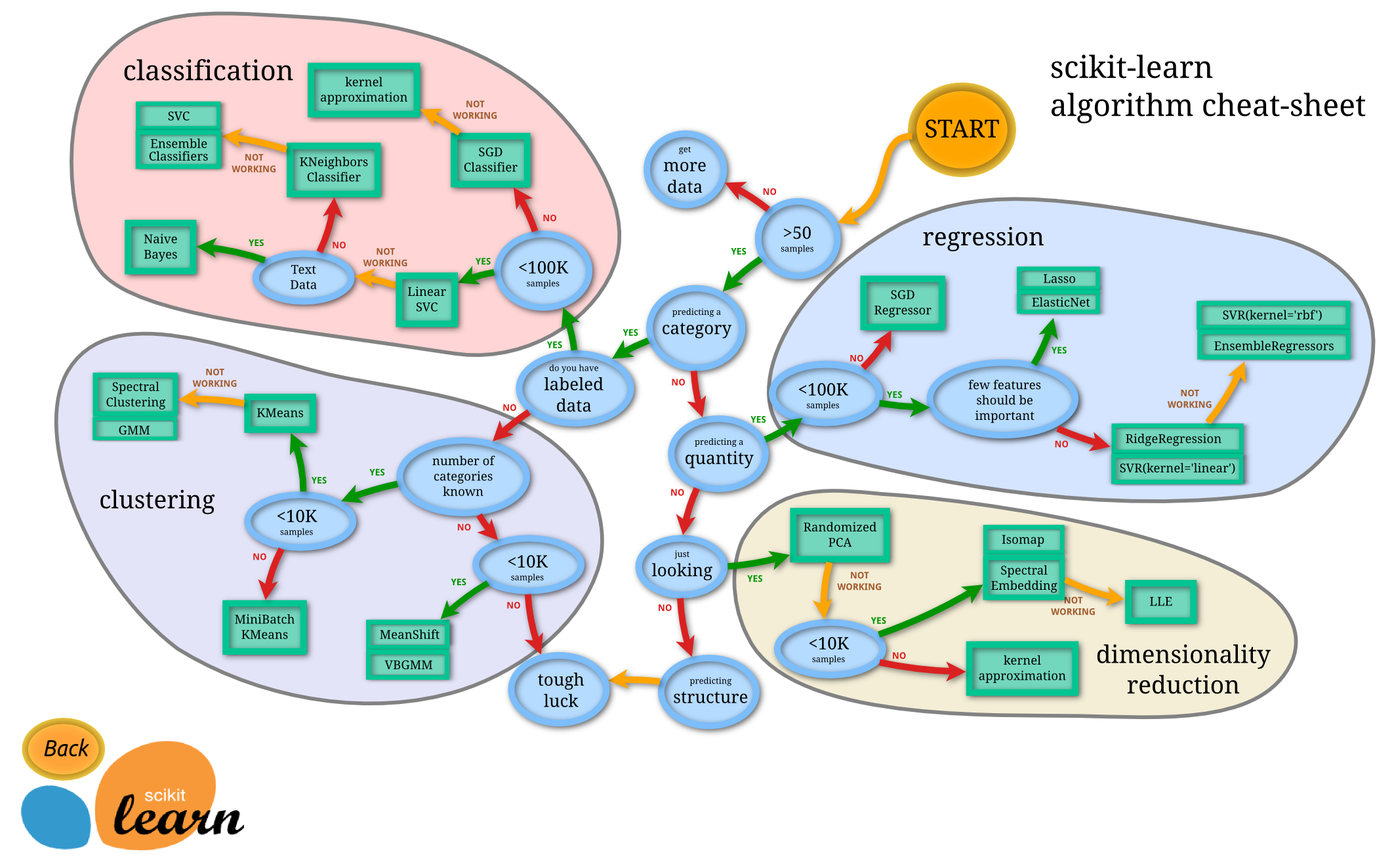
4.1 Mod: Selection
Toward selecting the right model, I need to determine what sort of variable we are predicting ($Y$). Some questions worth asking:
Do I have a label?
Yes, $Y$ takes on two values,
0and1indicating<=50kand>50krespectivelyIs the label discrete?
Yes, $Y$ exists in two states and not over a spectrum as a continuous variable
Do I have less than 100k observations?
Yes, I have 36,177 observations
Is this data textual?
No, this data is numerical and categorical defined specifically in their meanings (i.e. lacks the ambiguity of text data)
So, a model that predicts known categories (probability of known outcome, i.e. supervised learning with classification) is what I need.
SciKit-Learn offers this helpful decision path to guide me, but I will probably want to try other things as well.
4.2 Mod: Benchmark: Naive Bayes
The Naive Bayes Classifier will be used as a benchmark model for this work.
Bayes' Theorem is as such:
$$P\left(A|B\right) = \frac{P\left(B|A\right) \cdot P\left(A\right)}{P\left(B\right)}$$It is considered naive as it assumes each feature is independent of one another.
Bayes Theorem calculates the probability of an outcome (e.g. wether an individual recieves income exceeding 50k/yr), based on the joint probabilistic distributions of certain other events (e.g. any factors we include in the model).
As an example, I propose a model that always predicts an individual makes more than 50k/yr. This model has no false negatives; it has perfect recall (recall = 1).
Note: The purpose of generating a naive predictor is simply to show what a base model without any intelligence would look like. When there is no benchmark model set, getting a result better than random choice is a similar starting point.
4.2.1 Naive Bayes: Application
Since this model always predicts a 1:
- All true positives will be found (
1when1is true), equal to the sum of the label - False positives for this model are the difference between the number of all observations and those correctly predicted (
1when0is true) - No true negatives will be found (
0when0is true) as no0s are ever predicted - No false negatives are predicted (
0when1is true) as no0s are ever predicted
Note: I set $\beta = \frac{1}{2}$ as I want to penalize false positives being costly for CharityML. Recall the implications of setting the values of $\beta$ from before
4.3 Mod: Model Application Pipeline
It can be useful to establish a routine for aspects related to modeling. This allows for standard comparison of outcomes generated from the same process.
4.4 Mod: Logistic Regression
Logistic regression produces probabilites of independent variables indicating a dependent variable. The outcome of logistic regression is bound between 0 and 1 (i.e. $ h_{\theta}\left(X\right) \in \left[0,1\right]$).
$$ h_{\theta}\left(X\right) = P\left(Y=1 | X\right)= \left\{ \begin{array}{ll} y=1 & \frac{1}{1+e^{-\left(\theta^{T}X\right)}} \\ y=0 & 1 - \frac{1}{1+e^{-\left(\theta^{T}X\right)}} \\ \end{array} \right. $$With a cost function of: $$ cost\left(h_{\theta}\left(X\right)\right) = \left(h_{\theta}\left(X\right)\right) \cdot \left(1 - h_{\theta}\left(X\right)\right)$$
Deriving and Minimizing the Cost Function: How does $ cost\left(h_{\theta}\left(X\right)\right) = \left(h_{\theta}\left(X\right)\right) \cdot \left(1 - h_{\theta}\left(X\right)\right)$, fall out of $\frac{1}{1+e^{-\left(\theta^{T}X\right)}}$ ?
The following math involves a knowledge of some single variable differential calculus, $y = x^{n} \rightarrow \frac{\Delta y}{\Delta x} = -n\cdot x^{n-1}$, and the chain rule, $\frac{\Delta}{\Delta x}f\left(g\left(x\right)\right)= f'\left(g\left(x\right)\right) \cdot g'\left(x\right)$:
$$h\left(x\right) = \frac{1}{1+e^{-x}}$$$$\frac{\Delta h\left(x\right)}{\Delta x} = \frac{\Delta}{\Delta x}\left(1+e^{-x}\right)^{-1}$$$$\because \frac{\Delta}{\Delta x}x^{n} = -n\cdot x^{n-1} \wedge \frac{\Delta}{\Delta x}f\left(g\left(x\right)\right)= f'\left(g\left(x\right)\right) \cdot g'\left(x\right) \implies$$$$\frac{\Delta}{\Delta x}\left(1+e^{-x}\right)^{-1} = -\left(1+e^{-x}\right)^{-2}\left(-e^{-x}\right) = \frac{-e^{-x}}{-\left(1+e^{-x}\right)^{2}} = \frac{e^{-x}}{\left(1+e^{-x}\right)} \cdot \frac{1}{\left(1+e^{-x}\right)}$$$$= \frac{\left(1+e^{-x}\right)-1}{\left(1+e^{-x}\right)} \cdot \frac{1}{\left(1+e^{-x}\right)} = \left(\frac{1+e^{-x}}{1+e^{-x}} - \frac{1}{1+e^{-x}}\right)\cdot \frac{1}{1+e^{-x}}$$$$= \left(1-\frac{1}{1+e^{-x}}\right) \cdot \frac{1}{1+e^{-x}} = \left(1-h\left(x\right)\right) \cdot h\left(x\right) \square$$4.5 Mod: Random Forest
NEED: WRITEUP, VISUALIZE
4.6 Mod: Ada Boost
NEED: WRITEUP, VISUALIZE
4.7 Mod: Gradient Boost
NEED: WRITEUP, VISUALIZE
4.8 Mod: Extreme Gradient Boosting
NEED: WRITEUP, TUNING, VISUALIZE
Mod: 4.9 K-Nearest Neighbors
NEED: WRITEUP, TUNING, VISUALIZE
4.10 Comparison
NEED: VISUALIZATION
The Gradient Boosting Classifer evaluates at the highest F-0.5 score of 0.76 on the test set. The Random Forest Classifier may be overfitting, seeing the F-0.5 score on the training set vs the testing set compated to the rest of the models.
An important task when performing supervised learning is determining which features provide the most predictive power.
By focusing on the relationship between only a few crucial features and the target label, I can simplify my understanding of the phenomenon, which is most always a useful thing to do.
In the case of this project, that means I wish to identify a small number of features that most strongly predict whether an individual makes at most or more than $50,000.
The top-5 factors in predicting if a person makes more than 50k annually are:
- marital status being a a married civilian spouse
- capital gain
- education number
- capital loss
- age

4.10.3 Comp: Reduced Feature Model Performance
I can now compare how the model performs when I remove all features than those that contribute the larges amount of prediction power.
The prediction power is reduced, but this model trained much faster than with all of the factors. Because the predictive power is already not incredibly strong, this reduction in prediction power for a gain in speed doesn't seem worth it. If the data were much larger, orders of magnitude, I may change my evaluation.
At this point, I prefer the model with all factors, even if it is a little slower than with only the 5 most influential factors.
... and that's it!
What did I do:
- Built a model to predict if a person makes more than 50k annually
How did I do it:
- Evaluated data from the census
- Recieved
- Examined distributions
- Evaluated skew
- Evaluated relationships between factors
- Examined correlations and Thiel's Uncertainty Coefficient
- Determined a metric to evaluate a model's performance given this problem
- F-0.5 Score prefering a high precision model
- Transformed the data
- Logarithmic, Normalized
- Split and reordered the data
- Ensured distribution of positive and negative classes were similar to those in the initial data
- Trained a number of models and selected the most predictive, given the metric
- Selected Gradient Boosting Classifier
- Tested the model with reduced features and determined I would stick with the fully featured model
Deploying the model by saving and tying it to a software solution for a customer could be a useful next step.